Nanome now connects directly to Claude Code through the Model Context Protocol. Describe the structure and the figure you want, and Claude builds the workspace: selections, colors, measurements, and contact maps, all computed against the real coordinates.
The server ships with 47 tools covering projects, workspaces, scenes, components, annotations, entries, and export. Every one of them was exercised against a live structure before release.
Setup takes about two minutes.
Install
Add the server:
claude mcp add --transport http nanome https://workspaces.nanome.ai/mcpThis writes an entry into ~/.claude.json scoped to the current directory. To make Nanome available across every project, add the -s user flag:
claude mcp add -s user --transport http nanome https://workspaces.nanome.ai/mcp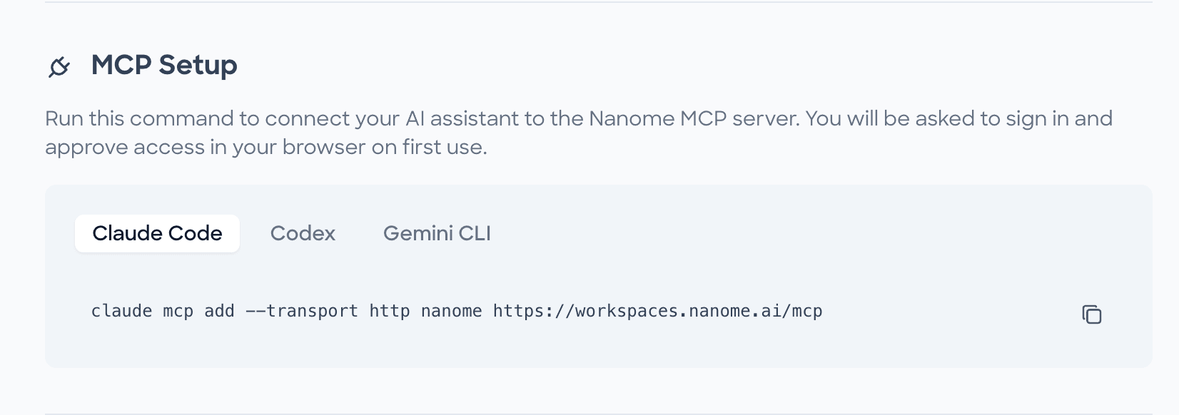
Authenticate
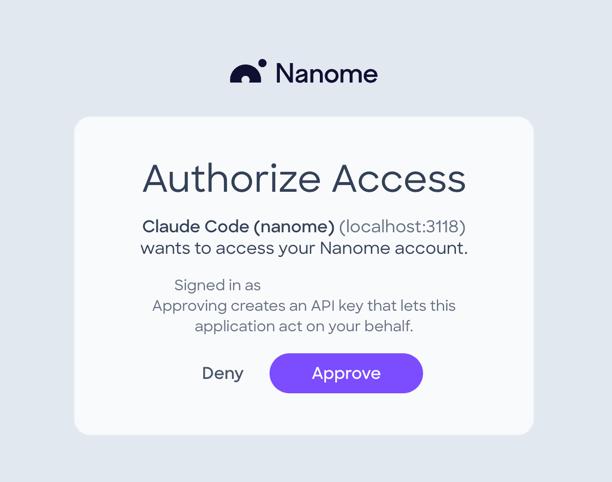
The server uses OAuth, with app.nanome.ai as the authorization server. Your existing Nanome credentials apply, and there is no separate account to create.
From the shell, in one command:
claude mcp login nanomeThe same flow runs from inside an interactive session:
claudeRun /mcp, select nanome, and choose Authenticate. Either path opens a browser window at app.nanome.ai for sign-in, and the token is stored on completion. Restart Claude Code afterward so the tools load into the session.
Verify
After adding the server, claude mcp list reports:
nanome: https://workspaces.nanome.ai/mcp (HTTP) - ✔ ConnectedThat status confirms the endpoint is reachable and speaks the MCP auth handshake. It does not confirm that authentication has completed. The reliable check is whether mcp__nanome__* tools appear in a fresh session.
What it looks like in practice
To test the server against something demanding, we built a walkthrough of KRAS G12C bound to sotorasib, PDB 6OIM.
KRAS is the most frequently mutated oncogene in human cancer, and it resisted drugging for 40 years. Its surface offers no obvious binding cleft, and its natural ligand GTP binds with picomolar affinity, which rules out competition at that site. Sotorasib reaches a different target: in tumors carrying the G12C mutation, glycine 12 becomes a cysteine positioned beside a pocket that only exists while the switch II loop is displaced. The drug occupies that transient pocket and forms a covalent bond to the cysteine. It was approved in 2021.
That makes it a useful test case, because the explanation has to travel from the whole protein, to a loop that shifts, to a pocket that exists only while it shifts, to a single bond.
Three prompts from the build are below. The full workspace contains nine scenes.
Loading and rendering the structure
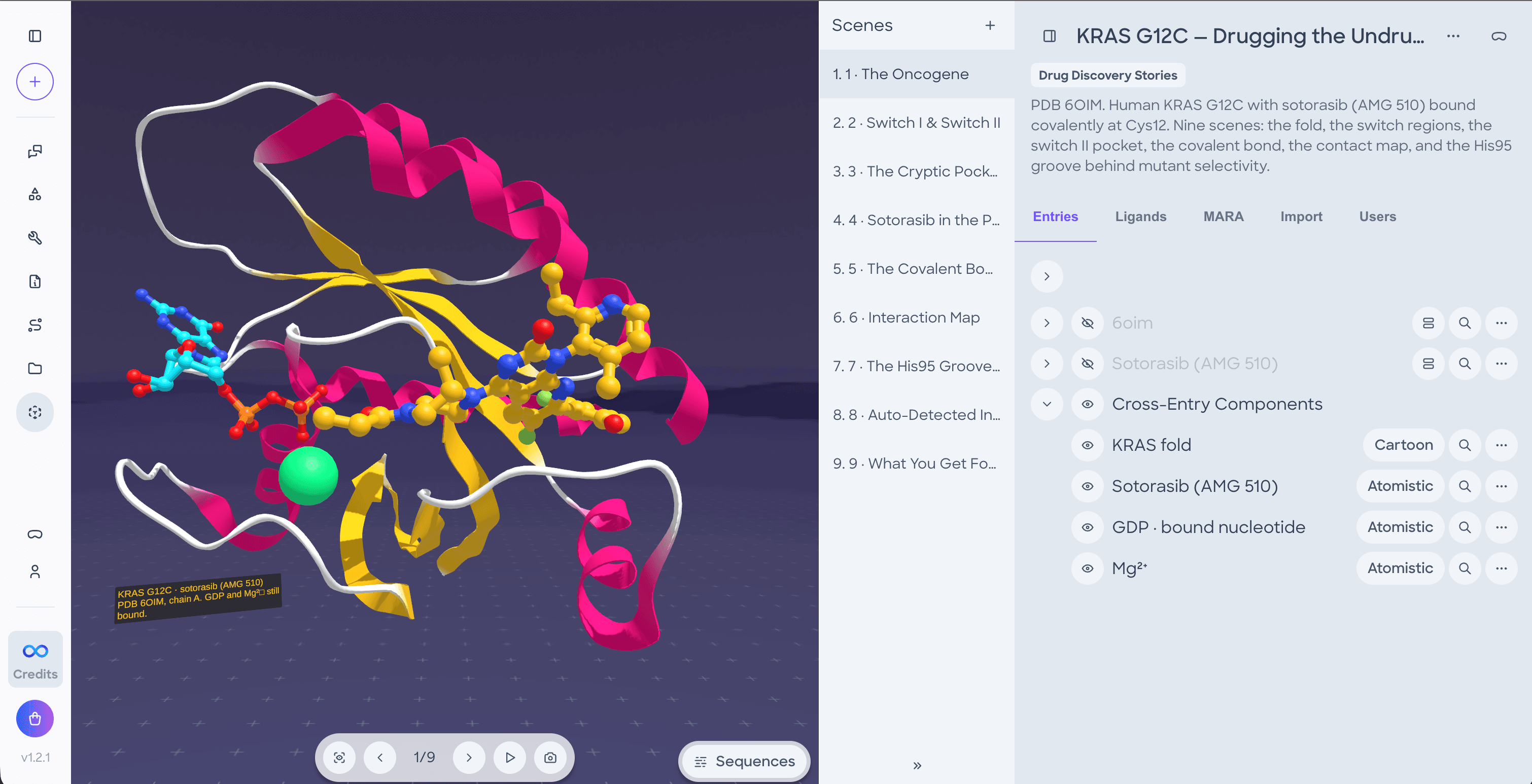
Pull up 6OIM, KRAS G12C with sotorasib bound. Show the fold as a cartoon
colored by secondary structure, put the drug in gold, and show me the
GDP and the magnesium.
Claude retrieved the structure from RCSB, requested an upload URL, posted the file, and assembled four components: a secondary-structure ribbon, the ligand with gold carbons against standard CPK heteroatoms, GDP in cyan, and the Mg²⁺ ion as a green sphere.
Two inferences happened without instruction. Claude identified "the drug" as residue MOV by listing the ligands in the entry and reading their molecular weights, and it applied the gold to carbons only, preserving conventional coloring for nitrogen and oxygen.
Selecting the binding pocket
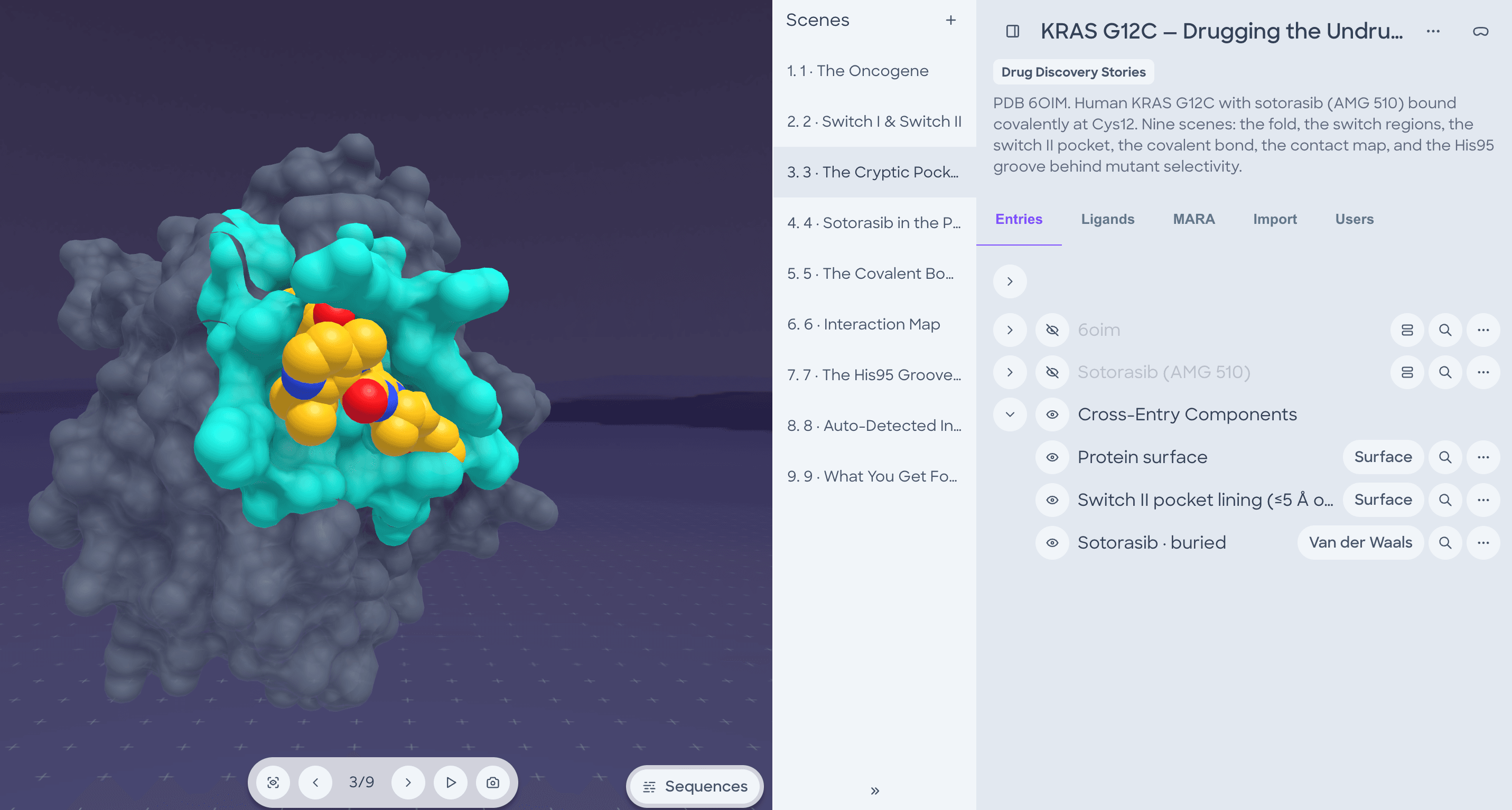
Surface the whole protein semi-transparent, and color everything within
5 Å of the ligand so I can see the switch II pocket.
The pocket lining resolved to a distance filter evaluated server-side against the deposited coordinates: every protein atom within 5 Å of the ligand, expanded to whole residues. For 6OIM that returns 21 residues.
No atom in that selection is named by hand. The same sentence produces the correct pocket for any structure, because the component stores a rule rather than a list.
Measuring the covalent bond
Show me the covalent bond. Cys12 and the acrylamide warhead big, the rest
of the ligand small. Measure the sulfur-carbon distance, the attack angle,
and the torsion.
Cys12 Sγ to sotorasib C25 measures 1.81 Å, a carbon-sulfur single bond read from the deposited coordinates.
All three measurement types accept flat atom lists: two serials for a distance, three for an angle with the vertex in the middle position, four for a dihedral. The acrylamide warhead was isolated by explicit atom serial, and the remainder of the ligand rendered thin and dim so attention falls on the bond.
These measurements are live annotations anchored to atoms rather than text written into a caption. They persist and update as the structure moves.
Explore the workspace
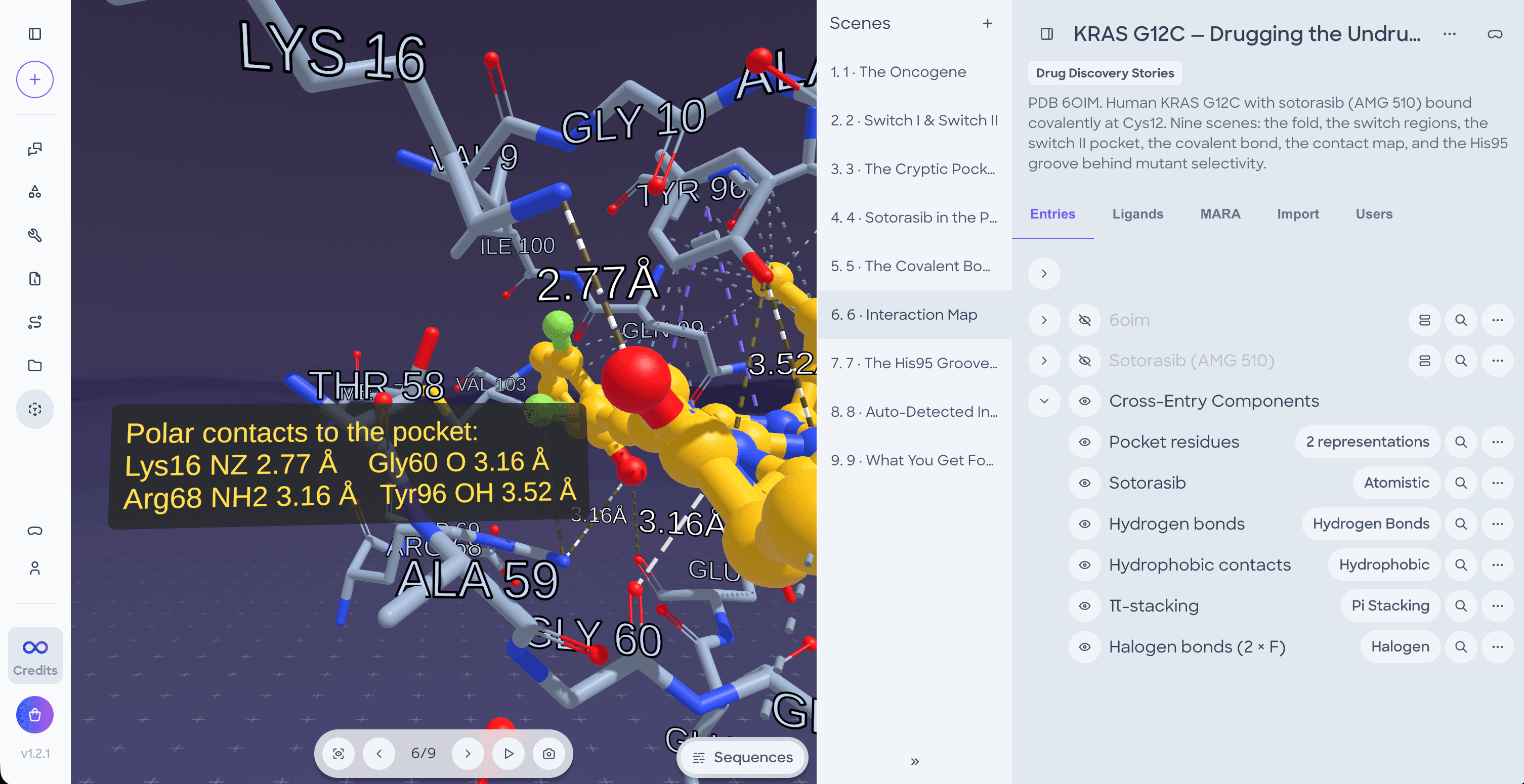
The remaining six scenes cover the switch I and switch II regions, the full ligand-pocket contact map with four measured hydrogen bonds, the His95 groove that accounts for mutant selectivity, and a scene built entirely from add_default_components to show the zero-configuration output.
Visit the public workspace here! It rewards walking through, particularly in headset, where the switch II pocket registers as a cavity with real depth.
Notes from the build
A few behaviors are worth knowing before you start.
add_interaction_components requires the ligand and the protein to occupy separate entries. A standard PDB deposits both as one entry, which produces the error "Cannot add cross-entry components entry and itself". Export the ligand to SDF and re-upload it as its own entry, after which the tool returns all eight contact types plus a pocket surface in a single call.
reset_default_components appends the default components and leaves existing custom components in place, rather than clearing the scene first.
export_component fails on smi for some ligands, returning "RDKit failed to generate SMILES". The same component exports correctly as sdf.
load_entry_from_content validates the three-line MOL header strictly. For files you did not generate, use request_entry_upload and post the file instead.
Atom serials map one-to-one onto PDB serials with no offset, which makes scripted figure generation considerably simpler.
Why this matters
The limiting factor in molecular design stopped being data some time ago. It is interface. Structures stay abstract until you can stand inside one, and a team that cannot see a mechanism ends up debating a picture of it.
An MCP server is a modest piece of engineering on its own. What it changes is the distance between describing a structure and having one. The sentence a scientist would say to a colleague is now the sentence that builds the workspace, and the result is something that colleague can open and turn around in their own hands.
The nine-scene walkthrough above took roughly 11 minutes to build.
Get started
claude mcp add --transport http nanome https://workspaces.nanome.ai/mcp
claude mcp login nanome
Restart Claude Code, then describe what you want to see.